What if we could only use named CSS colors on the web?

This question came to me one evening at work sometime last summer. I love programming and math, but my eye for design leaves some (okay... a lot) to be desired. When prototyping UI, I usually stick to the named CSS colors and wait for our design team to pick out some seemingly-random looking hex values that end up being perfectly complementary every time. If you saw some of my UI prototypes, your reaction to the above question would probably be something similar to, "Thank goodness we don't have to only use named CSS colors on the web".

A humorous thought, but this question stayed in my head. What would the web look like? What if we could only use named CSS colors on computers in general? What would the entire world look like in named CSS colors? Let's answer that question.

Formalization

The mathmatician in me immediately started to generalize this question. Colors are often represented (on a computer at least) as a combination of a red, blue, and green values. Each of these color values is an integral value bounded between 0 and 255. Let's formalize.

We define a color $C$ to be a 3-dimensional vector $\begin{bmatrix} r \\ g \\ b \end{bmatrix}$ with

$$r, g, b \in \mathbb{Z} \text{ and } 0 \leq r, g, b \leq 255$$

To answer our question, we need to take some sort of image and convert every color in the image to one of the named CSS colors. Given a set of colors $S$ (in this case, $S$ contains the named CSS colors) and a query color $C$, which color in $S$ do we change $C$ to? I decided to use the Euclidean distance to determine this (those familiar with color gamuts are taking their palms to their faces after reading that, because RGB colors are not linearly related, and thus the euclidean distance in RGB space does not mean what it does in, say, real 3D space. If I were repeating this experiment, I would first convert to HSV before doing any calculations, where I would get a more accurate result. For the purposes of demonstrating the effectiveness of a k-d tree, RGB color space will suffice). We can use some tools from real analysis to formalize this. We can define the set of all possible colors $E$ as a 3-dimensional metric space with our metric, $d: E \times E \mapsto \mathbb{R}$, being the standard Euclidean distance.

As a reminder, for n-dimensional vectors $d$ is defined as follows:

$$ d(\vec{x},\vec{y}) = \sqrt{\sum_{k=1}^{n} (x_{k} - y_{k})^2 } $$

We can now generalize our problem: given an n-dimensional metric space $E$, a set $S \subset E$, and a query point $q \in E$, what is the element $x \in S$ such that $\forall y \in S - \{ x \}$ we have $d(x,q) < d(y,q)$

In this generalization, $E$ is the metric space (treated as a set for breviy set) of all RGB colors, $S$ is the set of named CSS colors, $q$ is the query color in our image (that we must change to one of the named CSS colors), and $d$ is our Euclidean distance formula defined above.

As it turns out, this generalization is exactly the famous nearest neighbor problem. Finally we are getting to the title of this post...

Solving the problem

For a single query color $q$, its hard to get much better than naive linear search. We iterate through every named color in our set and calculate the distance from $q$ to the named color. The named color that produced the minimum distance from $q$ is our nearest neighbor, and the the new color for $q$. For a standard 4k image, this requires 8,294,400 iterations over our color set, with each iteration taking linear time on the number of colors in the set. Since there are 148 named colors in the latest CSS spec, we will be doing 1.1 billion queries to our distance function. This means 1.1 billion square roots and comparisons. That's not great... can we do better?

Astute readers will have realized that we don't actually need to perform any square root operations. If the distance between points A and B is greater than the distance between points A and C, then the distance squared between A and B will be greater than the distance squared between A and C. We don't care about the actual distance, just minimizing it. By taking out the square root, we have just saved quite a few clock cycles, but our algorithmic complexity has only improved by a constant amount. We can do much better than that.

If you read the title of this post, you have probably already realized that the applicaton of k-d trees is one solution.

A k-d tree looks pretty similar to a normal binary search tree, and familiarity with this data structure is assumed for the following discussion. Like a binary search tree, each node in our k-d tree has two children: the left node is "less" than its parent and the right node is "greater" than its parent. Defining less and greater is easy when working with real numbers (or 1-dimensional vectors), but is harder to define when we have more than one dimension. For example, is $\begin{bmatrix} 40 \\ 20 \\ 10 \end{bmatrix}$ greater or less than $\begin{bmatrix} 10 \\ 40 \\ 20 \end{bmatrix}$? Multi-dimensional vector spaces have no easily definable total order relation that would give us much use in coming to a solution to our problem. So then how do we adapt a binary search tree to higher dimensions? The answer initially appears quite simple: we isolate one dimension at a time and iterate through our dimensions at each level of our tree. At each level, operating on only a single dimension, we use the standard greater-than less-than relation that our binary search tree uses. This concept is easier to express in an example than in prose, so I will do just that:

Construction of a k-d tree

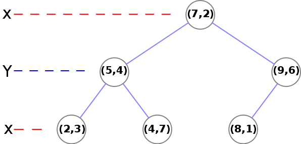
Consider the following six vectors, shamelessly stolen from an example on Wikipedia. These vectors are 2-dimensional, but the process for higher dimensions is exactly the same.

$$\begin{bmatrix} 5 \\ 4 \end{bmatrix} \begin{bmatrix} 2 \\ 3 \end{bmatrix} \begin{bmatrix} 8 \\ 1 \end{bmatrix} \begin{bmatrix} 9 \\ 6 \end{bmatrix} \begin{bmatrix} 7 \\ 2 \end{bmatrix} \begin{bmatrix} 4 \\ 7 \end{bmatrix}$$

Let's walk through the construction of a kd-tree. First we sort these vectors by their first dimension and ignore the other one. We now have, in order:

$$\begin{bmatrix} 2 \\ 3 \end{bmatrix} \begin{bmatrix} 4 \\ 7 \end{bmatrix} \begin{bmatrix} 5 \\ 4 \end{bmatrix} \begin{bmatrix} 7 \\ 2 \end{bmatrix} \begin{bmatrix} 8 \\ 1 \end{bmatrix} \begin{bmatrix} 9 \\ 6 \end{bmatrix}$$

We extract the median element and recurse on the left and right halves of the array after incrementing the dimension.

Sidenote: You may notice this process looks similar to quicksort; it is possible to build a static kd-tree in $O(n \cdot \log n)$ time if a $O(n)$ median finding algorithm is used to select a pivot and partition the array. I use a normal sorting algorithm to find my pivots due to the ease of implementation. This means the construction of my kd-tree is slightly slower at $O(n \cdot \log^2 n)$.

The median we have extracted is $\begin{bmatrix} 7 \\ 2 \end{bmatrix}$, which is placed as the root node of our k-d tree. For the right half of the array, we now sort by the second dimension and get:

$$\begin{bmatrix} 8 \\ 1 \end{bmatrix} \begin{bmatrix} 9 \\ 6 \end{bmatrix}$$

The case where we have only two elements is an end case. We take the first element and set it as the child of the previous node, and set the second element to be the left child of the first element.

Now, we recurse on the left side. We have

$$\begin{bmatrix} 2 \\ 3 \end{bmatrix} \begin{bmatrix} 5 \\ 4 \end{bmatrix} \begin{bmatrix} 4 \\ 7 \end{bmatrix}$$

Again we extract the median element ($\begin{bmatrix} 5 \\ 4 \end{bmatrix}$) and recurse on the left and right side. Both of these only have one node (another end case in our recursion) and the nodes are just set as the left and right children of their parent node.

Here is what the k-d tree looks like after construction:

Here is some python code for this construction. It may illuminate the construction process.

class Node(object):
	def __init__(self):
		self.left = None
		self.right = None
		self.dim = None
		self.val = None

def build_kdtree(vectors, node, dimension, max_dimension):
    vals = sorted(vectors, key=lambda v: v[dimension])
    if len(vals) == 1:
        node.val = vals[0]
        return node
    if len(vals) == 2:
        node.val = vals[1]
        node.left = Node()
        node.left.val = vals[0]
        return node
    mid = int((len(vals) - 1) / 2)
    node.val = vals[mid]
    node.left = build_kdtree(vals[:mid], Node(), (dimension+1) % max_dimension, max_dimension)
    node.right = build_kdtree(vals[mid+1:], Node(), (dimension+1) % max_dimension, max_dimension)
    return node

build_kdtree will return the root node in the constructed k-d tree.

Nearest neighbor on a k-d tree

Now that we have built our k-d tree we can search through it! Unfortunately, this is not as easy as searching through a binary search tree. Initially we follow a similar process as building the tree and continue down through the nodes (comparing only one dimension at a time) until we reach a leaf node (if this were normal binary search, we would be finished). We compute the distance squared of this leaf node and our query point and save this as our current best guess. Then we walk back up the tree. For each node that we move up, we perform the following steps:

1. Calculate the distance between the query point and the current node. If the distance is less than our current best guess, we update our best guess.
2. Check if any points exist on the other half of the tree rooted at the current node could be a better guess. Each node of our tree represents a split (or a partition) of space on a specified dimension (this is the comparison dimension we used earlier at this node). We know that every child node to the right of our current node has a greater value for the current dimension than our current node, and every child node on the left has a lesser value for the current dimension that our current node. This means that if the distance from our query point to the plane splitting the other child node (which we can calculate by taking the absolute value of the difference of our query point at the current dimension with the value of the current dimension of the other child node) is greater than our best guess distance, we can elimanate the entire subtree rooted on the other half of our current node. This is where the time savings of k-d trees come into play. In mathematical terms, we are checking if the hypersphere defined by our query point and our best guess distance intersects the hyperplane that defines the partition we established during our k-d tree construction. If there is no intersection, we know our nearest neighbor could not possibly be in that plane, so there is no point recurring into it.
3. If the distance we calculated in step 2 was less than our current best guess distance, we must recursively conduct our entire searching algorithm on the subtree rooted on the other side and compare the result with the current best guess. If it is less than our current best guess we update our current best guess. After this process (whether we updated our best guess or not), we continue unwinding our recursion.
   When this unwinding reaches the root node (and we perform the steps mentioned above on the root node), we have found our nearest neighbor! It is the point that gave us our current best guess.

Here is an excellent animation from Wikipedia user User A1 demonstrating this search process.

So is this really faster than the naive approach? For our case (specifically for lower dimensional spaces, like 3 dimensional for example) the answer is yes. On average, queries to k-d trees take $O(\log n)$ time, reasonably better than $O(n)$ time of the naive approach. For a 4k image, we can expect to do only 59 million queries to our distance function: substantial savings over the 1.1 billion queries required using the naive approach (note that we expect this many queries, but it will always be more in practice). Theoretically, this should be 20 times faster for 4k images (ignoring the cost of constructing our k-d tree, which is very low for only 148 nodes). If we were only restricting ourselves to 16 colors, we could expect a speedup of about 4 times. With 1000 colors in our k-d tree, we could expect a speedup of about 100 times. Theoretical savings don't always translate into real savings though. Let's see some results!

Results

I ran tests on a suite of images of varying sizes, from a small $283 \times 480$ pixel image to a massive $12285 \times 14550$ pixel image. These tests were run with a variety of color specifications: from the 16 colors in css1 to a random assortment of 64k colors. You can see the details for the tests I performed (as well as all the source code for the program) in this GitHub repository. As I write this, I still have tests running on even larger images. The largest and longest test will take an estimated 25 hours to run on my machine, so I will update with more results after the weekend.

The first test was performed on an image of Krumware's fearless leader: Colin Griffin.

So what would Colin look like if we could only see named CSS colors? Probably something like this:

The above image was generated in .14 seconds using the naive approach. The following image was also generated in .14 seconds, using the k-d tree method:

You may notice that the images are slightly different. These differences occur when a query point is equidistant from two points in our specification. Both algorithms will not update the color when it encounters a new distance that is equal in distance from the current one; since the k-d tree construction rearranges the order in which the points are reached, the algorithms may return different points for the same query (although both values are valid nearest neighbors).

Here is a chart comparing the runtimes on different color specifications:

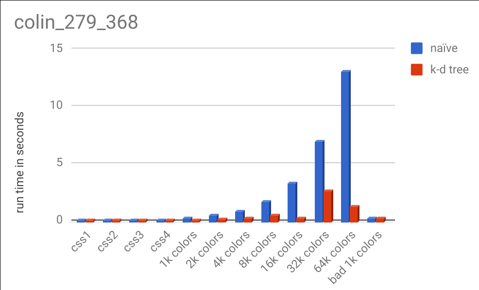
There are a lot of interesting results in this data. You can see that for large color specifications, the k-d tree algorithm handily outperformed the naive method, although not as much as our analysis predicted in theory. Computers are exceptionally good at iterating over lists of data and performing math on them (which is exactly what happens in the naive process) and CPUs have been optimized for decades to do this quickly. Cache misses had less of an imapact than I expected (you can see my full data here, which includes number of calls to the distance function, cache misses, number of instructions, and more). Due to the relative complexity of the k-d tree algorithm, it is easy to make mistakes that can cost precious CPU cycles. That coupled with the fact that I am a novice Rust programmer almost certainly led to slowdowns in the k-d tree code that could be optimized out (anybody who knows Rust, feel free to provide suggestions! My code is here).

From the chart above, you may also notice that the k-d tree took more time with 32k colors than it did with 64k colors. This was not a glitch and is deterministically repeatable. When performing this algorithm on the 32k color specification, there were 293,846,853 calls to the distance function. On the same image, but using the 64k color specification, there were only 136,309,021 about half as many. This is because with more colors, there is a chance that we can achieve a better distance guess earlier on in our search and not have to perform as many expensive recursive calls down other branches of our tree. Despite having a bigger tree (twice as large), we can eliminate more of the tree and end up saving computation time. This varies based on the image and the data set.

You may also notice the bad 1k colors column. I specifically constructed a color specification that would perform poorly with the k-d tree. The points are all one unit of distance away from every other point, so a lot of recursion has to happen to find the true nearest neighbor for a query point. If the dataset looks like this, the naive method always performs faster (due to the overhead of the k-d tree method).

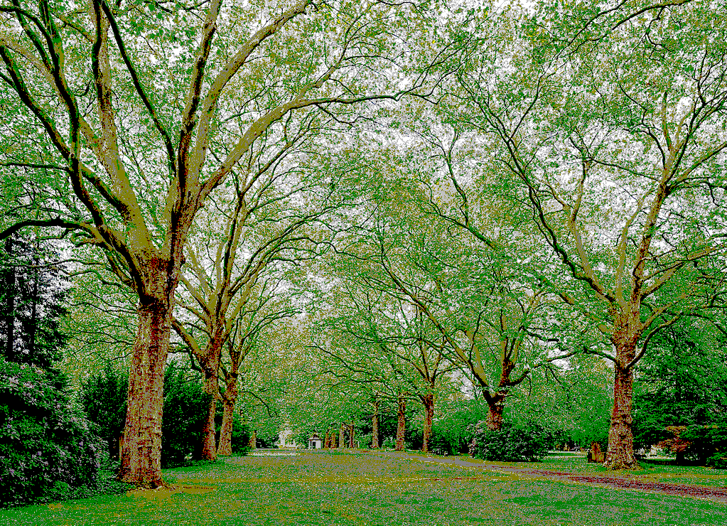
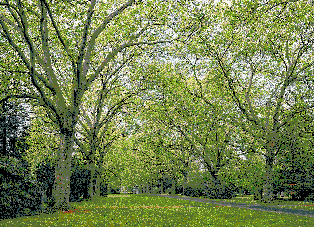
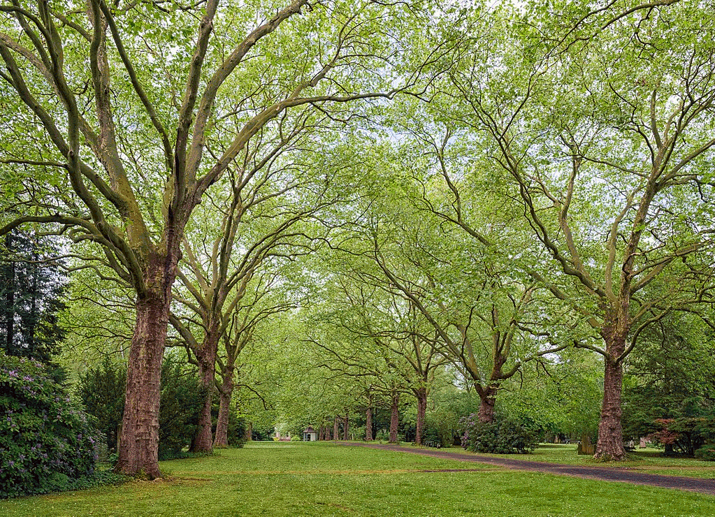
Colin's image is very handsome, but it doesn't have enough pixels in it to be interesting. Let's look at some larger images, harvested from Wikimedia Commons and published by Julian Herzog.

Original ($1023 \times 740$ pixels):

Using the 16 named CSS1 colors

Using the 148 named CSS4 colors

Using 2048 randomly selected colors

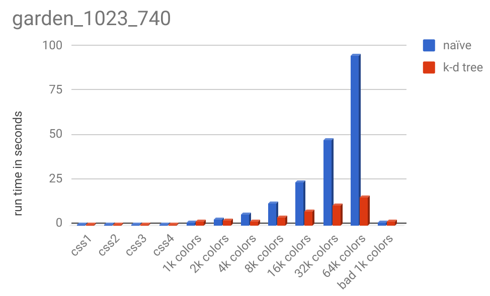
And here is the runtime chart:

Original ($1280 \times 720$ pixels)

Using the 16 named CSS1 colors

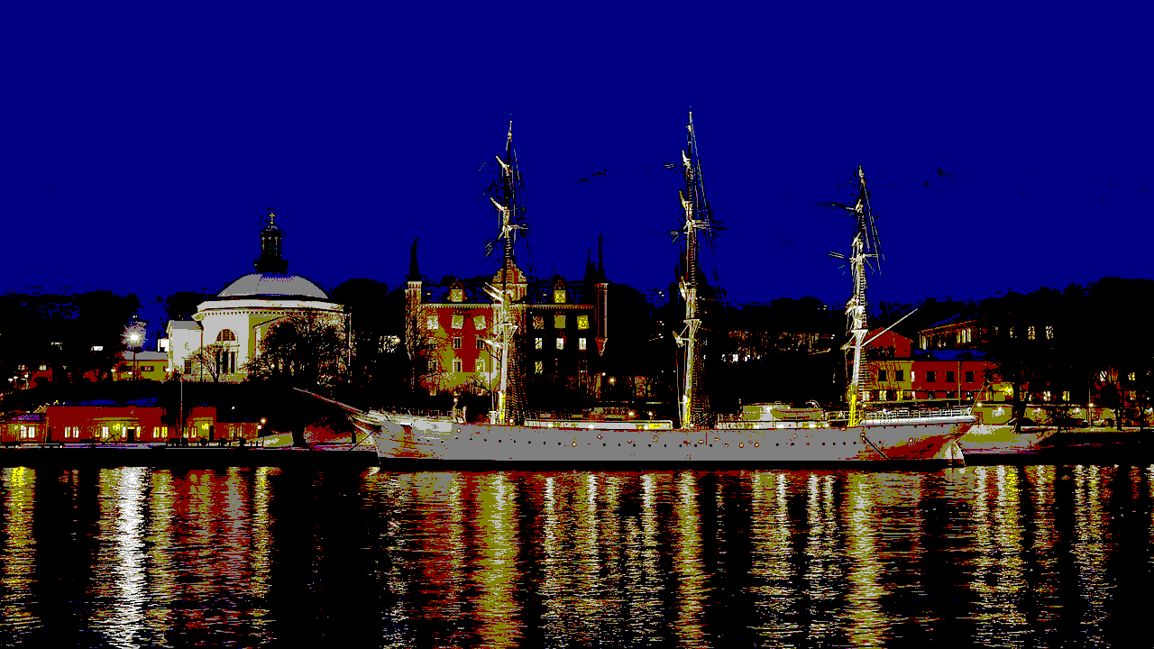
Using the 148 named CSS4 colors

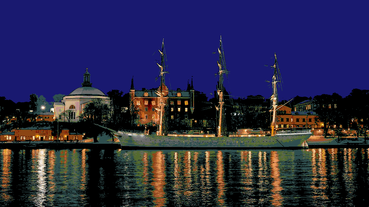
Using 4096 randomly selected colors

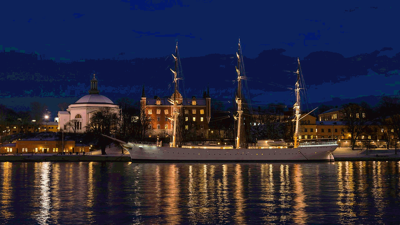
And here is the runtime chart:

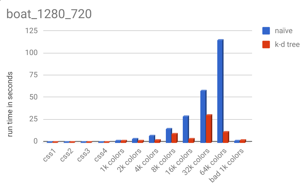
Notice the massive runtime decrease from 32k colors to 64k colors, 30.41 seconds to 11.00 seconds.

Original ($4096 \times 2304$ pixels, shown here scaled to 33%)

Using the 16 named CSS1 colors

Using the 148 named CSS4 colors

Using 1024 randomly selected colors (my personal favorite result)

Using 64k randomly selected colors

And here is the runtime chart:

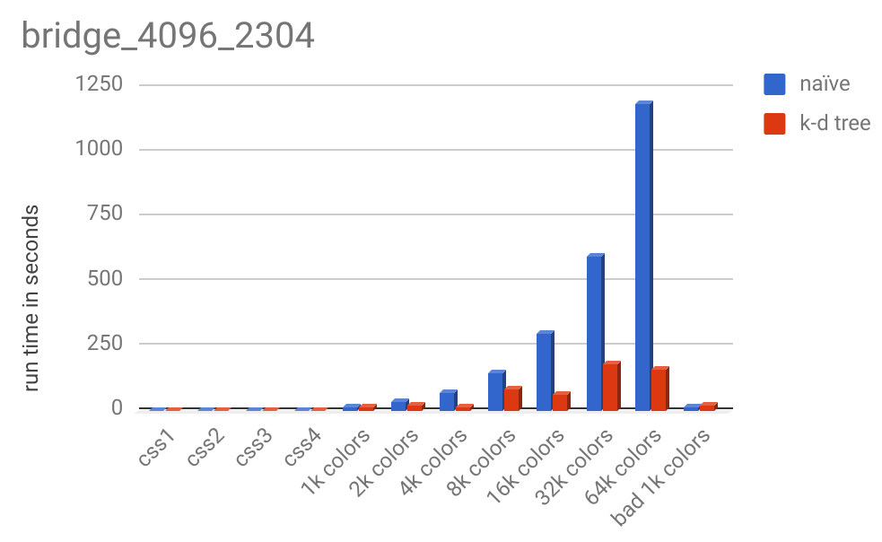
For images this large, the k-d tree significatnly outperforms the naive method. 64k colors took 1189 seconds (almost 20 minutes) while the k-d tree method took less than 3 minutes.

Now let's see how these algorithms perform on some exteremly large images. Google's Cultural Institute has some terrific high quality images of art pieces from around the globe. I used Johannes Vermeer's famous "Girl With a Pearl Earring" for this test. The image was a staggering $12285 \times 14550$ pixels, which took up 71M of space as a JPEG.

Original ($12285 \times 14550$ pixels, shown here scaled to 10%)

Using the 16 named CSS1 colors (24.47 seconds with k-d tree, 17.64 seconds naive)

Using the 148 named CSS4 colors (40.32 seconds with k-d tree, 64.94 seconds naive)

Using 32k randomly selected colors (1737.09 seconds (~29 minutes) with k-d tree, 11294.79 (~3.13 hours) seconds naive)

And of course, the runtime chart:

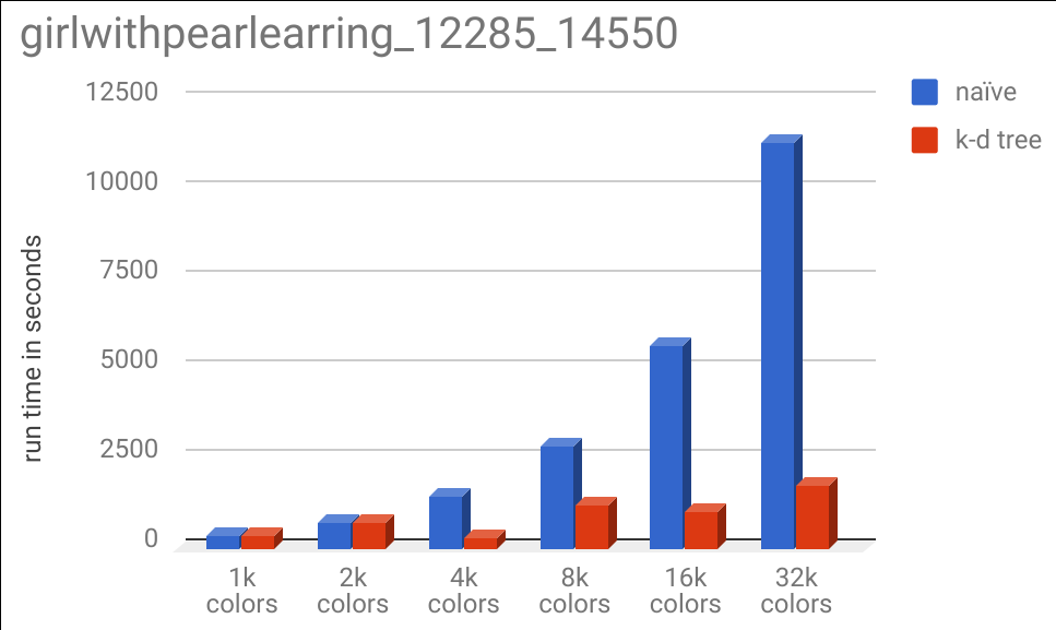
It is interesting to note that the 1k and 2k color specificatinos took almost the same run time for the k-d tree and naive implementations, but the 4k color specification took substantially less. This is due to the same effect described earlier, where adding more colors allows us to eliminate more of the tree from our search space as we recurse down the tree.

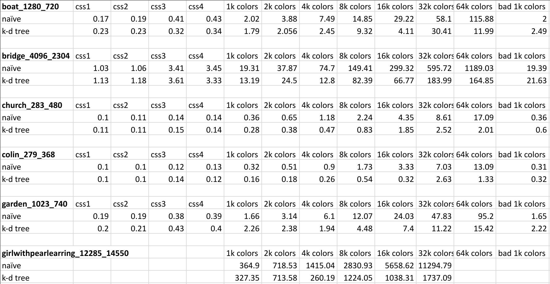
Here is a screenshot of the timing data that was used to generate the above charts:

Conclusion

The k-d tree method offered substantial performance benefits to the naive method, when the number of colors (or elements in our k-d tree) is large. This benefit is much more evident for large images, when the number of queries is large.

Did the k-d tree offer savings in all cases? No. The run time of the k-d tree code depended on the colors in our color specification, and the colors in the image. We could specifically construct color sets that would cause poor performance. The naive method's runtime depends only on the number of queries (or pixels in our image) and the number of colors in color specification. Thus we can accurately predict the runtime of the naive method, given the size of the image and the color specification.

Furthermore, when the number of colors in our color specification is small, the naive method often outperforms the k-d tree method. Even though the k-d tree method still makes fewer queries to the distance function, the overhead and complexity causes the runtime to be comprable or even greater than the naive method.

There are many other optimization strategies that could be used that I did not attempt. As images often use repeated color values for large regions, keeping a cache of the (say, 16 most) recently used colors and then checking through that first could offer large performance benefits, especially to the naive method. If I refine the algorithms, or if readers point out errors in my code or writing, I will update this post accordingly. I still have a few more tests running on some massive images, and I hope to get those published next week.

All source code and images and color specificationos can be found in this GitHub repo. If you have any questions or found any errors, please e-mail me at jadaytime (at) gmail.com. Unfortunately I can't send you a hexadecimal dollar, but I will be very grateful nonetheless. Thank you for reading!

UPDATE: Thanks to Bright Dru for pointing out an error in my k-d tree construction example.